The conventional approach

Usually when conducting an analysis of variance we follow the steps outlined below:

Step 1. Make model with multiple predictors no interaction.

Step 2. Make another model with the supposed interaction.

Step 3. anova(model1,model2), if the p-value is significant, the more complex model is the one that you should select.

The tidymodels approach

Let’s take a look at the Palmer Penguins dataset:

penguins %>% 
  head(5)

    # A tibble: 5 × 8
      species island    bill_length_mm bill_depth_mm flipper_length_mm body_mass_g
      <fct>   <fct>              <dbl>         <dbl>             <int>       <int>
    1 Adelie  Torgersen           39.1          18.7               181        3750
    2 Adelie  Torgersen           39.5          17.4               186        3800
    3 Adelie  Torgersen           40.3          18                 195        3250
    4 Adelie  Torgersen           NA            NA                  NA          NA
    5 Adelie  Torgersen           36.7          19.3               193        3450
    # ℹ 2 more variables: sex <fct>, year <int>

We have a few variables of interest which we can hypothesise may be interacting with each other. Let’s visualise the data:

penguins %>% 
  na.omit() %>% 
  ggplot(aes(bill_length_mm,bill_depth_mm))+
  geom_point(aes(color = species)) +
  geom_smooth(method = lm, color = "orange",
              formula = 'y~x',se=FALSE) + 
  geom_smooth(method = lm, aes(color = species),
              formula = 'y~x',
              se=FALSE) +
  labs(y="Bill Depth (mm)",
       x= "Bill Length (mm)")+
  theme_minimal()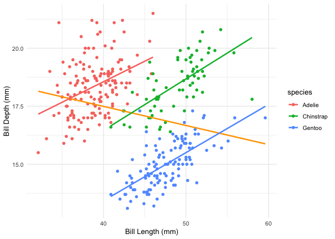

The general linear model doesn’t seem too bad, but it doesn’t take into account potential interactions between species and the variables above. Conventionally we would test this by comparing two models, one which accounts for the interaction and one that doesn’t:

model1 <- lm(bill_length_mm ~ bill_depth_mm * species, data = penguins %>% na.omit())
# summary(model1)

model2 <- lm(bill_length_mm ~ bill_depth_mm + species, data =  penguins %>% na.omit())
# summary(model2)

anova(model1, model2) %>%
  tidy() 

    # A tibble: 2 × 7
      term                          df.residual   rss    df sumsq statistic  p.value
      <chr>                               <dbl> <dbl> <dbl> <dbl>     <dbl>    <dbl>
    1 bill_length_mm ~ bill_depth_…         327 1954.    NA   NA       NA   NA      
    2 bill_length_mm ~ bill_depth_…         329 2095.    -2 -141.      11.8  1.17e-5

We see that the p-value is statistically significant, so we choose the model with the interaction term.

The tidymodels framework

Create the data splits and feature engineering recipes

Let’s now take the tidymodels approach to the same problem. We start by defining our data budget and splits:

set.seed(1234)
penguin_split <- initial_split(penguins %>% 
                                 na.omit(), strata = species, prop = 0.8)
penguin_train <- training(penguin_split)
penguin_test <- testing(penguin_split)

Next, we will define the respective pre-processing recipes, one with the interaction term and another without it:

# model without interaction:
rec_normal <- 
  recipe(bill_length_mm ~ bill_depth_mm + species,
         data=penguin_train) %>% 
  step_center(all_numeric_predictors())
# the model with interaction:
rec_interaction <- 
  rec_normal %>% 
  step_interact(~ bill_depth_mm:species)

Create the workflows

Now that we have our recipes we can proceed to create our respective workflows:

# Define the model
penguin_model <- 
  linear_reg() %>% 
  set_engine("lm") %>% 
  set_mode("regression")
# Workflows
# normal workflow:
penguin_wf <- 
  workflow() %>% 
  add_model(penguin_model) %>% 
  add_recipe(rec_normal)
# interaction workflow
penguin_wf_interaction <- 
  penguin_wf %>% 
  update_recipe(rec_interaction)

Let’s now fit our model to the data:

## Fitting
# use the last_fit() to make sure data is trained on 
# training dataset and evaluated on test dataset. 
penguin_normal_lf <- 
  last_fit(penguin_wf,
           split = penguin_split)

penguin_inter_lf <- 
  last_fit(penguin_wf_interaction,
           split = penguin_split)

    → A | warning: Categorical variables used in `step_interact()` should probably be avoided;
                   This can lead to differences in dummy variable values that are produced by
                   ?step_dummy (`?recipes::step_dummy()`). Please convert all involved variables
                   to dummy variables first.

    There were issues with some computations   A: x1
    There were issues with some computations   A: x1

The ANOVA part

Before we compare the models using the anova() function, we have to extract the fitted models from the respective workflows:

normalmodel <- penguin_normal_lf %>% extract_fit_engine()
intermodel <- penguin_inter_lf %>% extract_fit_engine()

anova(normalmodel,intermodel) %>%
  tidy()

    # A tibble: 2 × 7
      term                          df.residual   rss    df sumsq statistic  p.value
      <chr>                               <dbl> <dbl> <dbl> <dbl>     <dbl>    <dbl>
    1 ..y ~ bill_depth_mm + species         261 1657.    NA   NA       NA   NA      
    2 ..y ~ bill_depth_mm + specie…         259 1533.     2  124.      10.5  4.22e-5

We can get the model metrics using the yardstick package:

penguin_inter_lf %>% 
  collect_metrics()

    # A tibble: 2 × 4
      .metric .estimator .estimate .config        
      <chr>   <chr>          <dbl> <chr>          
      1 rmse    standard       2.49  pre0_mod0_post0
      2 rsq     standard       0.782 pre0_mod0_post0

Let’s take a deeper look at the interaction terms:

intermodel %>% 
  tidy()

    # A tibble: 6 × 5
      term                             estimate std.error statistic   p.value
      <chr>                               <dbl>     <dbl>     <dbl>     <dbl>
    1 (Intercept)                        37.9       0.310    122.   5.51e-231
    2 bill_depth_mm                       0.837     0.184      4.55 8.41e-  6
    3 speciesChinstrap                    8.42      0.590     14.3  1.85e- 34
    4 speciesGentoo                      14.3       0.663     21.6  5.98e- 60
    5 bill_depth_mm_x_speciesChinstrap    1.10      0.343      3.22 1.45e-  3
    6 bill_depth_mm_x_speciesGentoo       1.27      0.308      4.11 5.21e-  5

Finally it may be useful to plot the results:

# plot model predictions:
penguin_inter_lf %>% 
  collect_predictions() %>% 
  ggplot(aes(.pred, bill_length_mm)) +
  geom_point() +
  geom_abline(intercept = 0, slope = 1, color = "orange", size =1) +
  labs(x = "Predicted Bill Length",
       y = "Observed Bill Length",
       title = "R² plot") +
  theme_minimal()

    Warning: Using `size` aesthetic for lines was deprecated in ggplot2 3.4.0.
    ℹ Please use `linewidth` instead.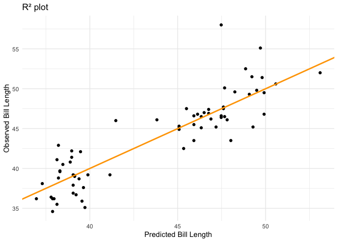

That’s it! We have successfully incorporated the tidymodels framework into the analysis ensuring robustness and sticking to good data practices.