Loading the data

This post explores the tidy Tuesday dataset for 2023-05-23, it is concerned with squirrel sightings in Central Park Let's load the data and take a quick look at it:

pacman::p_load(tidyverse,janitor,highcharter,leaflet) # Load relevant packages

squirrel <- readr::read_csv('https://raw.githubusercontent.com/rfordatascience/tidytuesday/master/data/2023/2023-05-23/squirrel_data.csv')

squirrel %>% 
  clean_names() -> squirrels

squirrels %>% 
  head(5)

# A tibble: 5 × 31
      x     y unique_squirrel_id hectare shift     date hectare_squirrel_number
  <dbl> <dbl> <chr>              <chr>   <chr>    <dbl>                   <dbl>
1 -74.0  40.8 37F-PM-1014-03     37F     PM    10142018                       3
2 -74.0  40.8 21B-AM-1019-04     21B     AM    10192018                       4
3 -74.0  40.8 11B-PM-1014-08     11B     PM    10142018                       8
4 -74.0  40.8 32E-PM-1017-14     32E     PM    10172018                      14
5 -74.0  40.8 13E-AM-1017-05     13E     AM    10172018                       5
# ℹ 24 more variables: age <chr>, primary_fur_color <chr>,
#   highlight_fur_color <chr>,
#   combination_of_primary_and_highlight_color <chr>, color_notes <chr>,
#   location <chr>, above_ground_sighter_measurement <chr>,
#   specific_location <chr>, running <lgl>, chasing <lgl>, climbing <lgl>,
#   eating <lgl>, foraging <lgl>, other_activities <chr>, kuks <lgl>,
#   quaas <lgl>, moans <lgl>, tail_flags <lgl>, tail_twitches <lgl>, …

Data Viz.

Lets plot the sightings along the latitude and longitude coordinates, to reveal where most of the sightings occur:

# squirrels %>% 
#   ggplot(aes(x,y))+
#   geom_point()+
#   theme_minimal()+
#   labs(x="Latitude",
#        y="Longitude") 
#   

squirrels %>% 
  rename(Longitude=y,
         Latitude=x) %>% 
hchart('scatter', hcaes(x = Latitude, y = Longitude), name = "Squirrel Sighting") %>% 
  hc_colors("#00AFBB") %>% 
  hc_title(text="Squirrel Sighting in Central Park")

There are alot of sigthtings, if you look closely we can see the outline of Central Park in the plot above. It would be interesting to see how this differs according to the primary color of the squirrel's fur. In other words, are squirrel with different fur color sighted in different regions of the park?

squirrel_by_col<- squirrels %>% select(x,y,primary_fur_color) %>% mutate(primary_fur_color = if_else(is.na(primary_fur_color),"Unknown",false = primary_fur_color))

squirrel_by_col  %>% 
ggplot(aes(x,y, color=primary_fur_color))+
  geom_point()+
  facet_wrap(~primary_fur_color)+
  theme_minimal()+
  scale_color_manual(values = c("#000000","#D2691E","#808080","#B2BEB5"))+
  labs(color="Primary Fur Color",
       y="Longitude",
       x="Latitude")+
  theme(legend.position = "bottom")

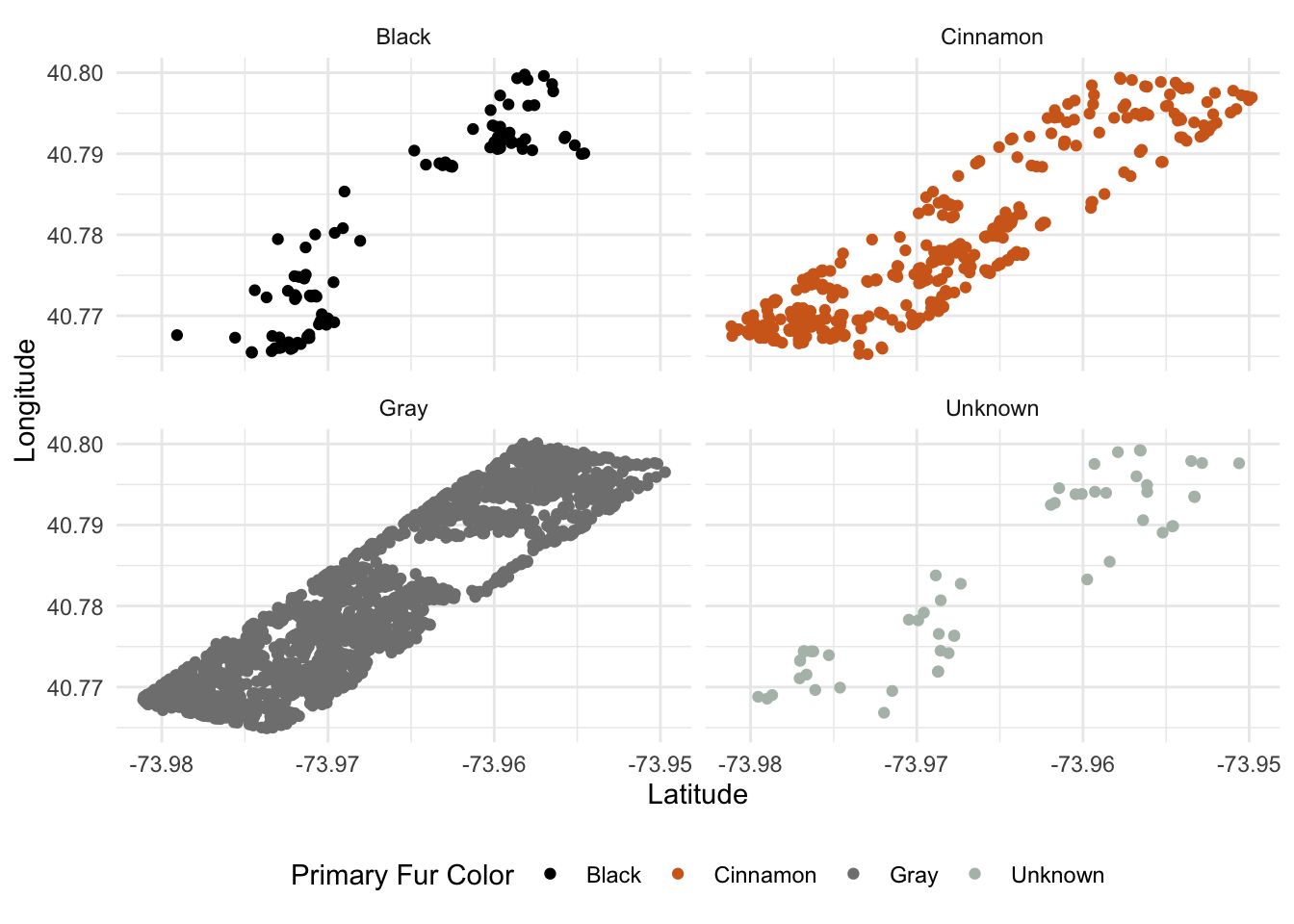
If we break down the visual by primary fur color, it becomes easier to see the sighting patterns. The squirrels with Gray as the primary fur color are seen the most and quite evenly across the whole park. There might be a body of water where we see the gap in sightings for those squirrels. The second category with the most sightings are squirrels with cinnamon as their primary color. Although not as concentrated as the gray, the sightings follow a similar pattern. The remaining two categories, black & unknown primary fur colors are sighted far more sporadically, concentrated mostly in the southwestern and north eastern parts of central park. Let's plot the data using leaflet to see if we can see any geographical patterns:

squirrels %>%
  filter(primary_fur_color == "Cinnamon") %>% # Filtered for cinnamon for quicker loading!
  select(x, y) %>%
  leaflet() %>% addTiles() %>%
  addMarkers( ~ x, ~ y)

It seems like our intuition was right, the gap in our plots corresponds to the outline of the Jacqueline Kennedy Onassis Resevoir. Now you know a bit more about squirrel sightings in Central Park!!