Loading the data

The data for this week's 2023-10-10 tidytuesday dataset is concerned with haunted places in the US. This post will focus on the geospatial elements of the data and will showcase how to deal with spatial elements as well as augment the tidytuesday dataset with other spatial datasets that will be required for visualisation. Various mapping techniques will be explored, adding some diversity to the post. Let's begin by loading the data and briefly looking at it:

pacman::p_load(tidyverse,RColorBrewer,cartogram,viridis,sf,echarts4r)

haunted_places <- readr::read_csv('https://raw.githubusercontent.com/rfordatascience/tidytuesday/master/data/2023/2023-10-10/haunted_places.csv')

haunted_places %>% 
  glimpse()

Rows: 10,992
Columns: 10
$ city           <chr> "Ada", "Addison", "Adrian", "Adrian", "Albion", "Albion…
$ country        <chr> "United States", "United States", "United States", "Uni…
$ description    <chr> "Ada witch - Sometimes you can see a misty blue figure …
$ location       <chr> "Ada Cemetery", "North Adams Rd.", "Ghost Trestle", "Si…
$ state          <chr> "Michigan", "Michigan", "Michigan", "Michigan", "Michig…
$ state_abbrev   <chr> "MI", "MI", "MI", "MI", "MI", "MI", "MI", "MI", "MI", "…
$ longitude      <dbl> -85.50489, -84.38184, -84.03566, -84.01757, -84.74518, …
$ latitude       <dbl> 42.96211, 41.97142, 41.90454, 41.90571, 42.24401, 42.23…
$ city_longitude <dbl> -85.49548, -84.34717, -84.03717, -84.03717, -84.75303, …
$ city_latitude  <dbl> 42.96073, 41.98643, 41.89755, 41.89755, 42.24310, 42.24…

We have a few data points of the haunted location, most notably longitude and latitude for the state and haunted location. Also have a brief description of the location and the location name.

Data Wrangling

We are interested in getting the number of haunted locations at the state level and comparing them to each other. In order to do so we will get the count at the state level. This can be done with the following:

haunted_places %>% 
  select(state,state_abbrev) %>%
  group_by(state,state_abbrev) %>% 
  count(name = "Haunted Places") %>%
  ungroup() -> state_counts

state_counts

# A tibble: 51 × 3
   state       state_abbrev `Haunted Places`
   <chr>       <chr>                   <int>
 1 Alabama     AL                        224
 2 Alaska      AK                         32
 3 Arizona     AZ                        156
 4 Arkansas    AR                        119
 5 California  CA                       1070
 6 Colorado    CO                        166
 7 Connecticut CT                        185
 8 Delaware    DE                         37
 9 Florida     FL                        328
10 Georgia     GA                        289
# ℹ 41 more rows

We now have a data frame with the state name, abbreviation and count of the haunted places. With this we are now ready to project this onto a map.

Data Visualisation

An interactive Choropleth

Although the data is now at the state level, we do not have any state border information. That information can be retrieved, it will be in JSON format. We can get it by using the jsonlite package:

json <- jsonlite::read_json("https://raw.githubusercontent.com/shawnbot/topogram/master/data/us-states.geojson")

The json object contains the border information for the states, this is how we will form the shapes of the choropleth map. We will need to use a combination of the json object and the aggregated state data in the functions of the echarts4r package:

state_counts |>
  e_charts(state) %>% 
  e_map_register("USA", json) %>% 
  e_map(`Haunted Places`, map = "USA") %>% 
  e_visual_map(
    `Haunted Places`, 
    inRange = list(color = c("#003f5c", "#bc5090","#ffa600"))) %>% 
  e_title(
    text = "Haunted Places in US States",
    subtext = "Data from tidytuesday"
  )
  

If you play around with the sliders you will see the data appear or dissapear depending on which direction you slide (top-bottom). It seems like California and Texas have a higher number of haunted places. If you hover over the state the name will appear and the slider value will change accordingly.

Cartogram

The previous visualisation used json, however R also has packages that allow us to use spatial data effectively, namely the sf package. The following 2 visualisations leverage the sf data type to make a cartogram and then a custom visualisation. Cartograms use normalisation to modify the geography, in essence the size of the map being created changes according to the variable being mapped. We begin by reading in a json file with the st_read() function which converts the file to sf in the importing process. We then make sure the object is consistent, convert it to the correct projection, merge it with the state_counts dataframe, and finally generate our normalised cartogram object and assign it to carto_data. These steps and sf object are shown below:

sf <- st_read("https://raw.githubusercontent.com/shawnbot/topogram/master/data/us-states.geojson")

sf_valid <- st_make_valid(sf) %>% 
  st_transform(5070) # Transform to a projected CRS (e.g., USA Contiguous Albers Equal Area Conic)

merged_data <- merge(sf_valid, state_counts, by.x = "name", by.y = "state")

carto_data <- cartogram_cont(merged_data, "Haunted Places", itermax=5)

Now that the sf object is ready, it can be plotted:

#| echo: false
ggplot(data = carto_data) + 
  geom_sf(aes(fill = `Haunted Places`)) +
  scale_fill_viridis(option = "A",labels =scales::comma)+
  theme_void() +
  labs(title = "",
       fill = "No. of Haunted\nPlaces") +
  theme(legend.position = "bottom",
        legend.key.height = unit(.2,"cm"),
        legend.direction = "horizontal",
        plot.title = element_text(hjust = 0.5, size = 20, face = "bold", margin = margin(b = 10)),
        legend.text = element_text(size = 8),
        legend.title =  element_text(size = 8, face = "bold")
  ) +
  guides(fill = guide_colorbar(title.position = "top", title.hjust = 0.5))+
  labs(title = "Haunted Places in US States") 

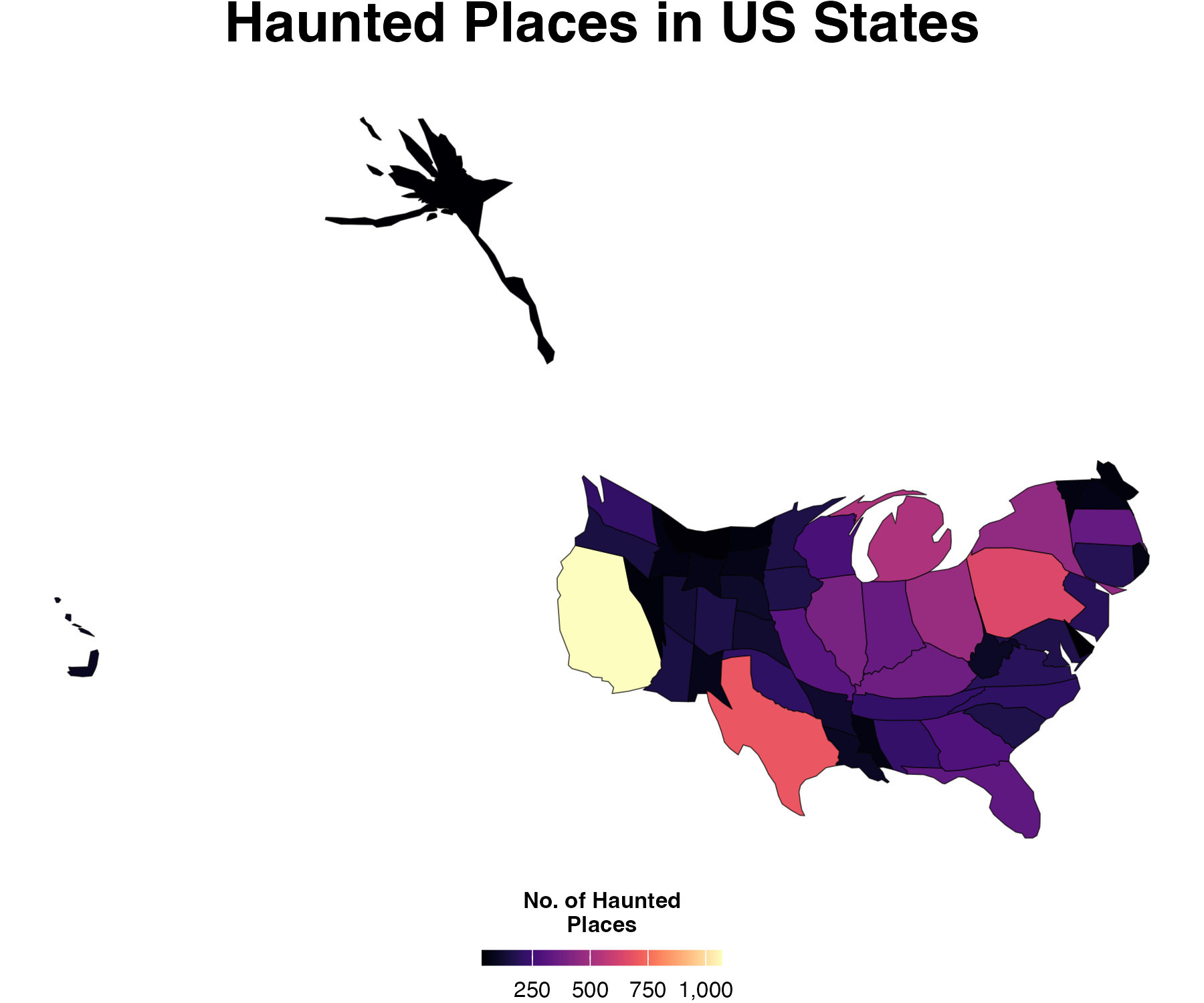
We can see that the shape of the map has changed, in fact the states have changed in size, in proportion to their value of haunted places. Therefore we see that California is bigger, states with low values have shrunk, like Alaska.

Lego Choropleth

For this final visualisation we will map the choropleth, however the twist will be that the states will be legos! Some initial set up is required for this. First, we create categories of the color hues, then a custom theme is created, finally we will use points/centroids as lego pices. This requires some wrangling and then joining to the dataset:

clean<-merged_data%>%
  mutate(clss=case_when(
    `Haunted Places`>0 &`Haunted Places` <200~"1",
    `Haunted Places`>201 & `Haunted Places`<400~"2",
    `Haunted Places`>401 & `Haunted Places`<600~"3",
    `Haunted Places`>601 & `Haunted Places`<800~"4",
    `Haunted Places`>801 & `Haunted Places`<1000~"5",
    TRUE~"6"
  ))

# Set color palette
pal <- c("#003f5c","#58508d","#bc5090","#ff6361","#ffa600","#005f73")
# Set color background
bck <- "#001219"

# Set theme 
theme_custom <- theme_void()+
  theme(
    plot.margin = margin(1,1,10,1,"pt"),
    plot.background = element_rect(fill=bck,color=NA),
    legend.position = "bottom",
    legend.title = element_text(hjust=0.5,color="white",face="bold"),
    legend.text = element_text(color="white")
  )


grd<-st_make_grid(
  clean, # map name 
  n = c(60,60) # number of cells per longitude/latitude
)%>%
  # convert back to sf object
  st_sf()%>%
  # add a unique id to each cell 
  # (will be useful later to get back centroids data)
  mutate(id=row_number())

# Extract centroids
cent<-grd%>%
  st_centroid()

# Intersect centroids with basemap
cent_clean<-cent%>%
  st_intersection(clean)

# Make a centroid without geom
# (convert from sf object to tibble)
cent_no_geom <- cent_clean%>%
  st_drop_geometry()

# Join with grid thanks to id column
grd_clean<-grd%>%

  left_join(cent_no_geom)

OK! we are ready to plot:

ggplot()+
  geom_sf(
    # drop_na() is one way to suppress the cells outside the country
    grd_clean %>% filter(!is.na(Haunted.Places)), 
    mapping=aes(geometry=geometry,fill=clss)
  )+
  geom_sf(cent_clean,mapping=aes(geometry=geometry),fill=NA,pch=21,size=0.5)+
  labs(fill="No. Haunted Places")+
  guides(
    fill=guide_legend(
      nrow=1,
      title.position="top",
      label.position="bottom"
    )
  )+
  scale_fill_manual(
    values=pal,
    label=c("0-200","201-400","401-600","601-800",">800", "1000+")
  )+
  theme_custom

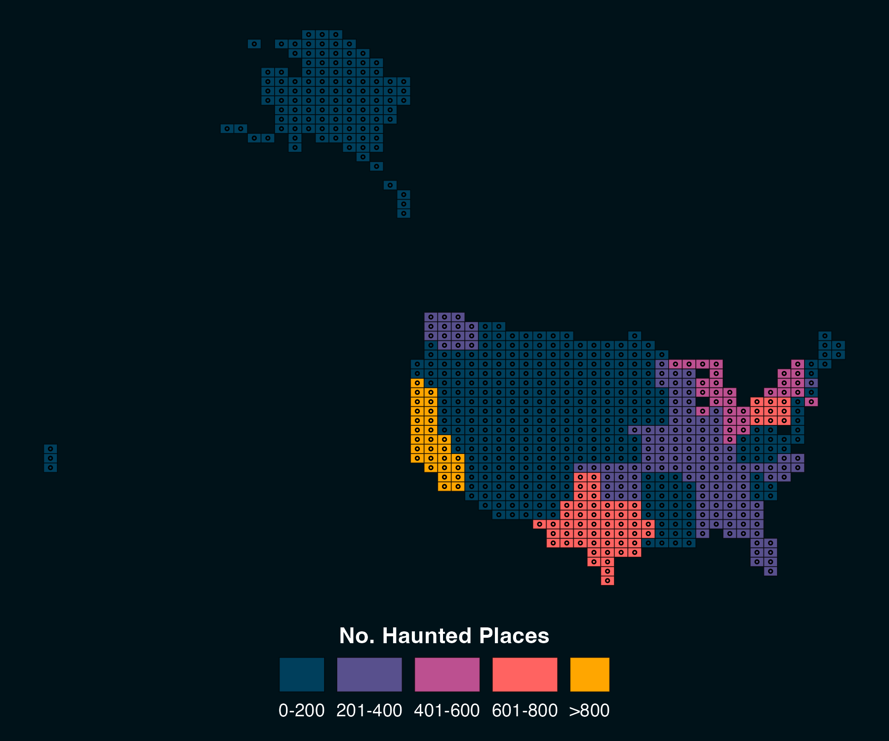
The plot looks neat! This blog touched on a few elements of dealing with spatial data and some visualisation techniques. How can you push the limit of your spatial data?!