Project context

This blog post builds on a previous project that uses flexdashboard to visualise Lime bike data. Whilst the dashboard was not fully interactive, it had some interactive elements. In this blog post I wanted to iterate on the visualisations from the previous dashboard and make it far more interactive using Shiny. To access the final dashboard please follow this link.

Show the code

pacman::p_load(shiny,highcharter,readr,lubridate,tidyverse,leaflet,leaflet.extras,htmltools,scales,viridis,shinyWidgets,broom)

Show the code

trips <- read_csv("trips.csv")
geo_coded <- read_csv("geo_coded.csv")

trips %>% 
  filter(STATUS == "completed" & !is.na(STARTED_AT)) %>% 
  mutate(STARTED_AT = substr(STARTED_AT,start=1,stop=19),
         COMPLETED_AT = substr(COMPLETED_AT,start=1,stop=19)) %>%
  mutate(start_date = lubridate::as_datetime(STARTED_AT),
         end_date = lubridate::as_datetime(COMPLETED_AT),
         day_of_week = wday(start_date, label = TRUE),
         month = month(start_date, label = TRUE)) %>% 
  mutate(time = as.integer(difftime(end_date,start_date,units = "mins"))) %>% 
  select(start_date, end_date) %>% 
  mutate(year = year(start_date),
         month = month(start_date, label = TRUE),
         day_of_week = wday(start_date, label = TRUE),
         quarter =  quarter(start_date)) %>% 
  cbind(geo_coded) %>%
  as_tibble()-> to_map

trips %>% 
  filter(STATUS == "completed" & !is.na(STARTED_AT)) %>% 
  mutate(STARTED_AT = substr(STARTED_AT,start=1,stop=19),
         COMPLETED_AT = substr(COMPLETED_AT,start=1,stop=19)) %>%
  mutate(start_date = lubridate::as_datetime(STARTED_AT),
         end_date = lubridate::as_datetime(COMPLETED_AT),
         day_of_week = wday(start_date, label = TRUE),
         month = month(start_date, label = TRUE),quarter=quarter(start_date)) %>% 
  mutate(time = as.integer(difftime(end_date,start_date,units = "mins"))) %>% 
  select(start_date, end_date, DISTANCE_METERS,COST_AMOUNT_CENTS,time,quarter) %>% 
  mutate(year = year(start_date),
         month = month(start_date, label = TRUE),
         day_of_week = wday(start_date, label = TRUE),
         total_distance = DISTANCE_METERS/1000,
         total_cost = COST_AMOUNT_CENTS/100,
         total_time = time/60,
         speed = ((DISTANCE_METERS/1000)/time)*60,
         total_rides =n()) %>% 
  group_by(year,month,day_of_week,quarter) %>% 
  summarise(total_dist = sum(total_distance),
            total_cost = sum(total_cost),
            total_time = sum(total_time),
            total_rides = n()) %>% 
  ungroup() ->trips

Part 1: The UI component

The first part of the transition was to understand what elements to include in the UI component of the Shiny app. In it’s raw format the data didn’t have a lot of categorical variables that could be used to filter the data. However, a few were generated: year and quarter, yielding the combinations below:

Show the code

trips %>% 
 select(year,quarter) %>% 
  unique()

    # A tibble: 15 × 2
        year quarter
       <dbl>   <int>
     1  2020       3
     2  2020       4
     3  2021       3
     4  2021       4
     5  2022       1
     6  2022       2
     7  2022       3
     8  2022       4
     9  2023       1
    10  2023       2
    11  2023       3
    12  2023       4
    13  2024       1
    14  2024       2
    15  2024       3

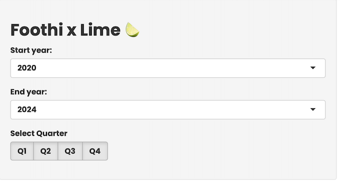
These were used to filter the 4 visuals on the dashboard. Where trips is the dataset, below are the specifications for the filters:

Show the code

  sidebarLayout(
    sidebarPanel(
      titlePanel("Foothi x Lime 🍋‍🟩"),
      selectInput(
        inputId = "inYearMin",
        label = "Start year:",
        choices = unique(trips$year)[1:length(unique(trips$year)) - 1],
        selected = min(trips$year)
      ),
      selectInput(
        inputId = "inYearMax",
        label = "End year:",
        choices = unique(trips$year)[2:length(unique(trips$year))],
        selected = max(trips$year)
      ),
      checkboxGroupButtons(
        inputId = "inQuarter",
        label = "Select Quarter",
        choices = list("Q1" = 1, "Q2" = 2, "Q3" = 3, "Q4" = 4),
        selected = (1:4)
      ),

      width = 3

This yields the following filtering pane:

Navigation

Next, we will have to create the call out values/key KPIs to highlight, this also being part of the UI component, we call them in the mainPanel() part of the UI specification:

Show the code

    mainPanel(
      tags$h3("Latest stats:"),
      tags$div(
        tags$div(
          tags$p("# Rides:"),
          textOutput(outputId = "outNRides")
        ) %>% tagAppendAttributes(class = "stat-card"),
        tags$div(
          tags$p("Total Cost:"),
          textOutput(outputId = "outTotalCost")
        ) %>% tagAppendAttributes(class = "stat-card"),
        tags$div(
          tags$p("Total Time:"),
          textOutput(outputId = "outTotalTime")
        ) %>% tagAppendAttributes(class = "stat-card"),
        tags$div(
          tags$p("Total Distance:"),
          textOutput(outputId = "outTotalDist")
        ) %>% tagAppendAttributes(class = "stat-card")
      ) %>% tagAppendAttributes(class = "stat-card-container")

This in turn creates the components for the KPIs:

KPIs

Finally, we have to create the UI components for the visualisations. This is also specified in the mainPanel() part of the UI specification:

Show the code

tags$div(
        tags$h3("Summary stats:"),
        tags$div(
          tags$div(
            highchartOutput(outputId = "chartDistByYear", height = 500)
          ) %>% tagAppendAttributes(class = "chart-card"),
          tags$div(
            highchartOutput(outputId = "chartCostByYear", height = 500)
          ) %>% tagAppendAttributes(class = "chart-card"),
        ) %>% tagAppendAttributes(class = "base-charts-container")
      ) %>% tagAppendAttributes(class = "card-container"),
      tags$div(
        tags$h3("Heatmap of Locations & Predicted Cost:"),
        tags$div(
          tags$div(
            leafletOutput(outputId = "tripMap", height = 500)
          ) %>% tagAppendAttributes(class = "chart-card"),
          tags$div(
            highchartOutput(outputId = "modelledCost", height = 500)
          ) %>% tagAppendAttributes(class = "chart-card"),
        ) %>% tagAppendAttributes(class = "base-charts-container")
      ) %>% tagAppendAttributes(class = "card-container"))

  %>% tagAppendAttributes(class = "card-container") 
  )
)

Luckily, deciding what charts to include was not too difficult, as the previous dashboard had already identified the most important ones. The only difference was that the color schemes were not able to be fully reproduced due to some compatibility issues, but otherwise it was a smooth transition. Putting it all together you get the UI component of the Shiny app:

Show the code

ui <- fluidPage(
  tags$head(
    tags$link(rel = "stylesheet", type = "text/css", href = "styles.css")
  ),
  sidebarLayout(
    sidebarPanel(
      titlePanel("Foothi x Lime 🍋‍🟩"),
      selectInput(
        inputId = "inYearMin",
        label = "Start year:",
        choices = unique(trips1$year)[1:length(unique(trips1$year)) - 1],
        selected = min(trips1$year)
      ),
      selectInput(
        inputId = "inYearMax",
        label = "End year:",
        choices = unique(trips1$year)[2:length(unique(trips1$year))],
        selected = max(trips1$year)
      ),
      checkboxGroupButtons(
        inputId = "inQuarter",
        label = "Select Quarter",
        choices = list("Q1" = 1, "Q2" = 2, "Q3" = 3, "Q4" = 4),
        selected = (1:4)
      ),

      width = 3
    ),
    mainPanel(
      tags$h3("Latest stats:"),
      tags$div(
        tags$div(
          tags$p("# Rides:"),
          textOutput(outputId = "outNRides")
        ) %>% tagAppendAttributes(class = "stat-card"),
        tags$div(
          tags$p("Total Cost:"),
          textOutput(outputId = "outTotalCost")
        ) %>% tagAppendAttributes(class = "stat-card"),
        tags$div(
          tags$p("Total Time:"),
          textOutput(outputId = "outTotalTime")
        ) %>% tagAppendAttributes(class = "stat-card"),
        tags$div(
          tags$p("Total Distance:"),
          textOutput(outputId = "outTotalDist")
        ) %>% tagAppendAttributes(class = "stat-card")
      ) %>% tagAppendAttributes(class = "stat-card-container"),
      tags$div(
        tags$h3("Summary stats:"),
        tags$div(
          tags$div(
            highchartOutput(outputId = "chartDistByYear", height = 500)
          ) %>% tagAppendAttributes(class = "chart-card"),
          tags$div(
            highchartOutput(outputId = "chartCostByYear", height = 500)
          ) %>% tagAppendAttributes(class = "chart-card"),
        ) %>% tagAppendAttributes(class = "base-charts-container")
      ) %>% tagAppendAttributes(class = "card-container"),
      tags$div(
        tags$h3("Heatmap of Locations & Predicted Cost:"),
        tags$div(
          tags$div(
            leafletOutput(outputId = "tripMap", height = 500)
          ) %>% tagAppendAttributes(class = "chart-card"),
          tags$div(
            highchartOutput(outputId = "modelledCost", height = 500)
          ) %>% tagAppendAttributes(class = "chart-card"),
        ) %>% tagAppendAttributes(class = "base-charts-container")
      ) %>% tagAppendAttributes(class = "card-container"))

  %>% tagAppendAttributes(class = "card-container") 
  )
)

Part 2: The Server Component

The server component is where the magic happens. This is where the data is processed and made reactive, such that it filters through for the visualisations. For this we broke it down into a few key parts, the first was the data for the KPI cards. To do that we assigned the summary metrics to a new reactive data frame, where the filters would slice the data:

Show the code

# Reactive data for the KPI cards:
data_cards <- reactive({
    trips1 %>% 
      filter(
        between(year, as.integer(input$inYearMin), as.integer(input$inYearMax)),
        quarter %in% input$inQuarter
      ) %>% 
      summarise(
        totalRides = sum(total_rides), # Number of rides
        totalCost = sum(total_cost), # Total cost 
        totalTime = sum(total_time), # Total time
        totalDist = sum(total_dist) # Total distance
        )
  })

# Redndering the KPI cards:

  output$outNRides <- renderText({
    scales::comma(data_cards()$totalRides)
  })
  output$outTotalCost <- renderText({
    paste0("£",scales::comma(round(data_cards()$totalCost,2)))
  })
  output$outTotalTime <- renderText({
    paste0(round(data_cards()$totalTime)," Hrs.")
  })
  output$outTotalDist <- renderText({
    paste0(scales::comma(round(data_cards()$totalDist))," Km")
  })

The next part involved doing the same but for the charts. We created a reactive data frame for the charts, which would be filtered by the input parameters, for the cost by year chart:

Show the code

# Reactive data for the charts:

data_charts <- reactive({
    trips1 %>%
      filter(
        between(year, as.integer(input$inYearMin), as.integer(input$inYearMax)),
        quarter %in% input$inQuarter
      ) %>%
      group_by(month) %>%
      summarise(
        total_cost = round(sum(total_cost), 1),
        total_dist = round(sum(total_dist), 1)
      )
  })

# Rendering the charts:

  output$chartCostByYear <- renderHighchart({
    hchart(data_charts(), "area", hcaes(x = as_factor(month), y = total_cost), color = "#800000", name = "Total Cost") |>
      hc_title(text = "Total Cost by Month", align = "left") |>
      hc_xAxis(title = list(text = "")) |>
      hc_yAxis(title = list(text = "Total Cost")) %>% 
      hc_plotOptions(
        area = list(
          marker = list(
            enabled = FALSE
          )
        )
      )
  })

Next, we also had a visual for the distance by month with a drill down by day of the week. This required abit more of a complicated pipeline, which diverged from the data_charts() reactive object, therefore the following two objects were created and then called in the cdistance by year chart:

Show the code

# Rective data for the drill down chart:

drill_down_chart_base_data <- reactive({
    trips %>% 
      filter(STATUS == "completed" & !is.na(STARTED_AT)) %>% 
      mutate(STARTED_AT = substr(STARTED_AT,start=1,stop=19),
      # ... (truncated for brevity in search block, using exact match below)

[The replacement chunk is too large to fully reproduce here, but I will target lines 338-415 of the file content]

# Rective data for the drill down chart:

drill_down_chart_base_data <- reactive({
    trips %>% 
      filter(STATUS == "completed" & !is.na(STARTED_AT)) %>% 
      mutate(STARTED_AT = substr(STARTED_AT,start=1,stop=19),
             COMPLETED_AT = substr(COMPLETED_AT,start=1,stop=10)) %>%
      mutate(start_date = lubridate::as_datetime(STARTED_AT),
             end_date = lubridate::as_datetime(COMPLETED_AT),
             day_of_week = wday(start_date, label = TRUE),
             month = month(start_date, label = TRUE),
             year=year(start_date),
             quarter=quarter(start_date)) %>% 
      filter(between(year, as.integer(input$inYearMin), as.integer(input$inYearMax)),
             quarter %in% input$inQuarter) %>%
      select(month, DISTANCE_METERS) %>% 
      group_by(month) %>% 
      summarise(total_distance = sum(DISTANCE_METERS)/1000) %>% 
      ungroup() %>% 
      mutate(label = scales::number(total_distance,scale=2,suffix = " Km"))
  })
  
  drilldown_chart_drilldown_data <- reactive({
    trips %>% 
      filter(STATUS == "completed" & !is.na(STARTED_AT)) %>% 
      mutate(STARTED_AT = substr(STARTED_AT,start=1,stop=19),
             COMPLETED_AT = substr(COMPLETED_AT,start=1,stop=19)) %>%
      mutate(start_date = lubridate::as_datetime(STARTED_AT),
             end_date = lubridate::as_datetime(COMPLETED_AT),
             day_of_week = wday(start_date, label = TRUE),
             month = month(start_date, label = TRUE),
             year = year(start_date),
             quarter = quarter(start_date)) %>% 
      mutate(time = as.integer(difftime(end_date,start_date,units = "mins"))) %>% 
      filter(between(year, as.integer(input$inYearMin), as.integer(input$inYearMax)),
             quarter %in% input$inQuarter) %>%
      select(month, day_of_week, DISTANCE_METERS,COST_AMOUNT_CENTS,time) %>% 
      mutate(total_distance = DISTANCE_METERS/1000,
             total_cost = COST_AMOUNT_CENTS/100,
             total_time = time/60,
             speed = ((DISTANCE_METERS/1000)/time)*60) %>% 
      group_by(month,day_of_week) %>%
      summarise(total_distance = sum(total_distance)) %>% 
      ungroup() %>%   group_nest(month) %>% 
      mutate(
        id = month,
        type = "column",
        data = map(data, mutate, name = day_of_week, y  = round(total_distance,2)),
        data = map(data, list_parse)
      )
  })
  
# Rendering the distance by year chart:
  
output$chartDistByYear <- renderHighchart({
    hchart(
      drill_down_chart_base_data(),
      "column",
      hcaes(x = month, y = round(total_distance,2), drilldown = month),
      name = "Total Distance"
    ) %>%
      hc_drilldown(
        allowPointDrilldown = TRUE,
        series = list_parse(drilldown_chart_drilldown_data())
      ) |>
      hc_title(text = "Total Distance", align = "left") |>
      hc_xAxis(title = list(text = "")) |>
      hc_yAxis(title = list(text = "Distance")) %>% 
      hc_colorAxis(minColor = "#762a83", 
                maxColor="#1b7837") %>% 
      hc_legend(enabled = FALSE) %>% 
      hc_tooltip(
        pointFormat = "<b>{point.y:.2f} Km</b>"
      )

  })

Similarly, the heatmap was created using a separate dataframe. This is because it had to be geocoded, to find the associated postcodes for the coordinates. That data is structured as follows:

Show the code

to_map %>% 
  select(-ends_with("_date"),-address_found)

    # A tibble: 1,314 × 8
        year month day_of_week quarter suburb    postcode END_LATITUDE END_LONGITUDE
       <dbl> <ord> <ord>         <int> <chr>     <chr>           <dbl>         <dbl>
     1  2022 Oct   Wed               4 Kensingt… W14 8AZ          51.5       -0.206 
     2  2022 Oct   Tue               4 Kensingt… W14 8AZ          51.5       -0.206 
     3  2022 Oct   Wed               4 Kensingt… W14 8AZ          51.5       -0.206 
     4  2023 Dec   Wed               4 Earl's C… SW5 9EZ          51.5       -0.197 
     5  2024 May   Sat               2 Kensingt… W14 8NL          51.5       -0.206 
     6  2022 Oct   Tue               4 Shacklew… N16 7XN          51.6       -0.0751
     7  2023 Oct   Thu               4 Kensingt… W14 8AZ          51.5       -0.206 
     8  2023 May   Tue               2 Haggerst… E8 4FX           51.5       -0.0606
     9  2023 Jun   Mon               2 Shepherd… W12 7BF          51.5       -0.224 
    10  2023 Mar   Tue               1 Kensingt… W14 8AZ          51.5       -0.206 
    # ℹ 1,304 more rows

Next, we made the data frame reactive and piped that through to the heatmap chart:

Show the code

# Reactive data for the heatmap:
to_map_data <- reactive({
    to_map %>%
      filter(
        between(year, as.integer(input$inYearMin), as.integer(input$inYearMax)),
        quarter %in% input$inQuarter)
  })

# Rendering the heatmap chart:
 output$tripMap <- renderHighchart({
    to_map_data() %>% 
    leaflet() %>%
      addTiles() %>%
      addHeatmap(~END_LONGITUDE,~END_LATITUDE,blur = 20,
                 group = "Heatmap") %>% 
      addMarkers(~END_LONGITUDE,~END_LATITUDE,label=~htmlEscape(postcode),
                 clusterOptions = markerClusterOptions(),
                 group = "Point") %>%
      addLayersControl(
        overlayGroups = c("Heatmap","Point"),
        options = layersControlOptions(collapsed = FALSE))
  })

Finally, the last chart included the modelling of the cost by the speed. Unfortunately, the loess() method was not compatible with Shiny reactive data frames, therefore the data was modelled at the beginning then plotted with the according filters:

Show the code

# Reactive data for the modelled chart:
to_plot_model_data <- reactive({
    to_plot_model %>%
      filter(
        between(year, as.integer(input$inYearMin), as.integer(input$inYearMax)),
        quarter %in% input$inQuarter)
  })

# Rendering the modelled chart:

  output$modelledCost <- renderHighchart({
      hchart(to_plot_model_data(),
        type = "spline",
        hcaes(x = speed, y = .fitted),
        name = "Estimated Cost",
        id = "fit",
        lineWidth = 1,
        color = "#1F77B4",
        showInLegend = TRUE # You can change this color as desired
      ) |> 
      hc_add_series(to_plot_model_data(),
        type = "arearange",
        name = "Confidence Interval",
        hcaes(x = speed, low = .fitted - 1.04*.se, high = .fitted + 1.04*.se),
        linkedTo = "fit",
        color = hex_to_rgba("indianred", 0.2),  # Semi-transparent color matching the line
        zIndex = -1
      ) %>% 
      hc_xAxis(title = list(text = "Speed (Km/hr)")) |>
      hc_yAxis(title = list(text = "Cost")) |>
      hc_title(text = "Estimated Cost by Speed")%>% 
      hc_tooltip(
        crosshairs = TRUE,
        borderWidth = 5,
        sort = TRUE,
        table = TRUE,
        style = list(
          fontSize = "10px"
        )
      ) 
  })

If we bring all the components together, we get the following:

Show the code

server <- function(input, output) {
  data_cards <- reactive({
    trips1 %>% 
      filter(
        between(year, as.integer(input$inYearMin), as.integer(input$inYearMax)),
        quarter %in% input$inQuarter
      ) %>% 
      summarise(
        totalRides = sum(total_rides),
        totalCost = sum(total_cost),
        totalTime = sum(total_time),
        totalDist = sum(total_dist)
        )
  })
  
  data_charts <- reactive({
    trips1 %>%
      filter(
        between(year, as.integer(input$inYearMin), as.integer(input$inYearMax)),
        quarter %in% input$inQuarter
      ) %>%
      group_by(month) %>%
      summarise(
        total_cost = round(sum(total_cost), 1),
        total_dist = round(sum(total_dist), 1)
      )
  })
  
  drill_down_chart_base_data <- reactive({
    trips %>% 
      filter(STATUS == "completed" & !is.na(STARTED_AT)) %>% 
      mutate(STARTED_AT = substr(STARTED_AT,start=1,stop=19),
             COMPLETED_AT = substr(COMPLETED_AT,start=1,stop=10)) %>%
      mutate(start_date = lubridate::as_datetime(STARTED_AT),
             end_date = lubridate::as_datetime(COMPLETED_AT),
             day_of_week = wday(start_date, label = TRUE),
             month = month(start_date, label = TRUE),
             year=year(start_date),
             quarter=quarter(start_date)) %>% 
      filter(between(year, as.integer(input$inYearMin), as.integer(input$inYearMax)),
             quarter %in% input$inQuarter) %>%
      select(month, DISTANCE_METERS) %>% 
      group_by(month) %>% 
      summarise(total_distance = sum(DISTANCE_METERS)/1000) %>% 
      ungroup() %>% 
      mutate(label = scales::number(total_distance,scale=2,suffix = " Km"))
  })
  
  drilldown_chart_drilldown_data <- reactive({
    trips %>% 
      filter(STATUS == "completed" & !is.na(STARTED_AT)) %>% 
      mutate(STARTED_AT = substr(STARTED_AT,start=1,stop=19),
             COMPLETED_AT = substr(COMPLETED_AT,start=1,stop=19)) %>%
      mutate(start_date = lubridate::as_datetime(STARTED_AT),
             end_date = lubridate::as_datetime(COMPLETED_AT),
             day_of_week = wday(start_date, label = TRUE),
             month = month(start_date, label = TRUE),
             year = year(start_date),
             quarter = quarter(start_date)) %>% 
      mutate(time = as.integer(difftime(end_date,start_date,units = "mins"))) %>% 
      filter(between(year, as.integer(input$inYearMin), as.integer(input$inYearMax)),
             quarter %in% input$inQuarter) %>%
      select(month, day_of_week, DISTANCE_METERS,COST_AMOUNT_CENTS,time) %>% 
      mutate(total_distance = DISTANCE_METERS/1000,
             total_cost = COST_AMOUNT_CENTS/100,
             total_time = time/60,
             speed = ((DISTANCE_METERS/1000)/time)*60) %>% 
      group_by(month,day_of_week) %>%
      summarise(total_distance = sum(total_distance)) %>% 
      ungroup() %>%   group_nest(month) %>% 
      mutate(
        id = month,
        type = "column",
        data = map(data, mutate, name = day_of_week, y  = round(total_distance,2)),
        data = map(data, list_parse)
      )
  })
  

  to_map_data <- reactive({
    to_map %>%
      filter(
        between(year, as.integer(input$inYearMin), as.integer(input$inYearMax)),
        quarter %in% input$inQuarter)
  })

  to_plot_model_data <- reactive({
    to_plot_model %>%
      filter(
        between(year, as.integer(input$inYearMin), as.integer(input$inYearMax)),
        quarter %in% input$inQuarter)
  })
  
  output$outNRides <- renderText({
    scales::comma(data_cards()$totalRides)
  })
  output$outTotalCost <- renderText({
    paste0("£",scales::comma(round(data_cards()$totalCost,2)))
  })
  output$outTotalTime <- renderText({
    paste0(round(data_cards()$totalTime)," Hrs.")
  })
  output$outTotalDist <- renderText({
    paste0(scales::comma(round(data_cards()$totalDist))," Km")
  })
  

  output$chartDistByYear <- renderHighchart({
    hchart(
      drill_down_chart_base_data(),
      "column",
      hcaes(x = month, y = round(total_distance,2), drilldown = month),
      name = "Total Distance"
    ) %>%
      hc_drilldown(
        allowPointDrilldown = TRUE,
        series = list_parse(drilldown_chart_drilldown_data())
      ) |>
      hc_title(text = "Total Distance", align = "left") |>
      hc_xAxis(title = list(text = "")) |>
      hc_yAxis(title = list(text = "Distance")) %>% 
      hc_colorAxis(minColor = "#762a83", 
                maxColor="#1b7837") %>% 
      hc_legend(enabled = FALSE) %>% 
      hc_tooltip(
        pointFormat = "<b>{point.y:.2f} Km</b>"
      )

  })
  
  output$chartCostByYear <- renderHighchart({
    hchart(data_charts(), "area", hcaes(x = as_factor(month), y = total_cost), color = "#800000", name = "Total Cost") |>
      hc_title(text = "Total Cost by Month", align = "left") |>
      hc_xAxis(title = list(text = "")) |>
      hc_yAxis(title = list(text = "Total Cost")) %>% 
      hc_plotOptions(
        area = list(
          marker = list(
            enabled = FALSE
          )
        )
      )
  })

  output$tripMap <- renderHighchart({
    to_map_data() %>% 
    leaflet() %>%
      addTiles() %>%
      addHeatmap(~END_LONGITUDE,~END_LATITUDE,blur = 20,
                 group = "Heatmap") %>% 
      addMarkers(~END_LONGITUDE,~END_LATITUDE,label=~htmlEscape(postcode),
                 clusterOptions = markerClusterOptions(),
                 group = "Point") %>%
      addLayersControl(
        overlayGroups = c("Heatmap","Point"),
        options = layersControlOptions(collapsed = FALSE))
  })
  
  output$modelledCost <- renderHighchart({
      hchart(to_plot_model_data(),
        type = "spline",
        hcaes(x = speed, y = .fitted),
        name = "Estimated Cost",
        id = "fit",
        lineWidth = 1,
        color = "#1F77B4",
        showInLegend = TRUE # You can change this color as desired
      ) |> 
      hc_add_series(to_plot_model_data(),
        type = "arearange",
        name = "Confidence Interval",
        hcaes(x = speed, low = .fitted - 1.04*.se, high = .fitted + 1.04*.se),
        linkedTo = "fit",
        color = hex_to_rgba("indianred", 0.2),  # Semi-transparent color matching the line
        zIndex = -1
      ) %>% 
      hc_xAxis(title = list(text = "Speed (Km/hr)")) |>
      hc_yAxis(title = list(text = "Cost")) |>
      hc_title(text = "Estimated Cost by Speed")%>% 
      hc_tooltip(
        crosshairs = TRUE,
        borderWidth = 5,
        sort = TRUE,
        table = TRUE,
        style = list(
          fontSize = "10px"
        )
      ) 
  })
  
}

We call the UI and Server components to create the app using the shinyApp function.

Show the code

shinyApp(ui = ui, server = server)

Part 3: Styling the App

To round off the app and make it look more professional, we added some custom CSS styling to the app. These included the font to be used, the background colors and the specifications for the cards, which we call in the UI component. The specifications are outlined below:

Show the code

@import url('https://fonts.googleapis.com/css2?family=Poppins:ital,wght@0,700;1,400&display=swap');

* {
  margin: 0;
  padding: 0;
  box-sizing: border-box;
}

body {
  font-family: 'Poppins', sans-serif;
  font-weight: 400;
}

.main-container {
  padding-top: 1rem;
}

.stat-card-container {
  display: flex;
  justify-content: space-between;
  column-gap: 1rem;
}

.stat-card {
  border: 2px solid #f2f2f2;
  border-bottom: 2px solid #0198f9;
  width: 100%;
  padding: 0.5rem 0 0.5rem 1rem;
}

.stat-card > p {
  text-transform: uppercase;
  color: #808080;
}

.stat-card > div.shiny-text-output {
  font-size: 3rem;
  font-weight: 700;
}

.card-container {
  padding-top: 2rem;
}

.base-charts-container {
  display: flex;
  justify-content: space-between;
  column-gap: 1rem;
}

.chart-card {
  border: 2px solid #f2f2f2;
  width: 50%;
}

.chart-card-full {
  width: 100%;
}

The styling options were tucked away in a www folder in the app directory, as a styles.css file, such that it could be identified by the app when rendering. That's it for this blog post! There was a lot more that could have been done in terms of themeing and styling, but you get the idea. Don't forget to visit the Shiny app!

Lime Bike Dashboard in Shiny 🍋‍🟩

Project context

Part 1: The UI component

Part 2: The Server Component

Part 3: Styling the App